Candidate-to-candidate Comparison
Comparing the Total Amount of Contributed Dollars and Unique Donors Sliced by Enriched Attributes
Overview
The previous sections demonstrated different approaches to the data and introduced useful SQL queries. We now introduce useful tools to compare donations sliced by the enriched attributes:
- Gender
- Age
- Ethnicity
- Federal state
- Median household income per county
Easy access and comprehensive charting is available through the e.ventures Data Cohort Analysis Google Sheet and the ObservableHQ.com notebook collection. Those interfaces fetch the data from the SQL Interface, thus, the same data can be downloaded using the SQL Interface /query endpoint.
Slicing the Contribution Data in the e.ventures Cohort Analysis Google Sheet
The Google Sheet focuses on the analysis of monthly donor cohorts and their attributes. The sheet also covers several other useful non cohort-related charts.

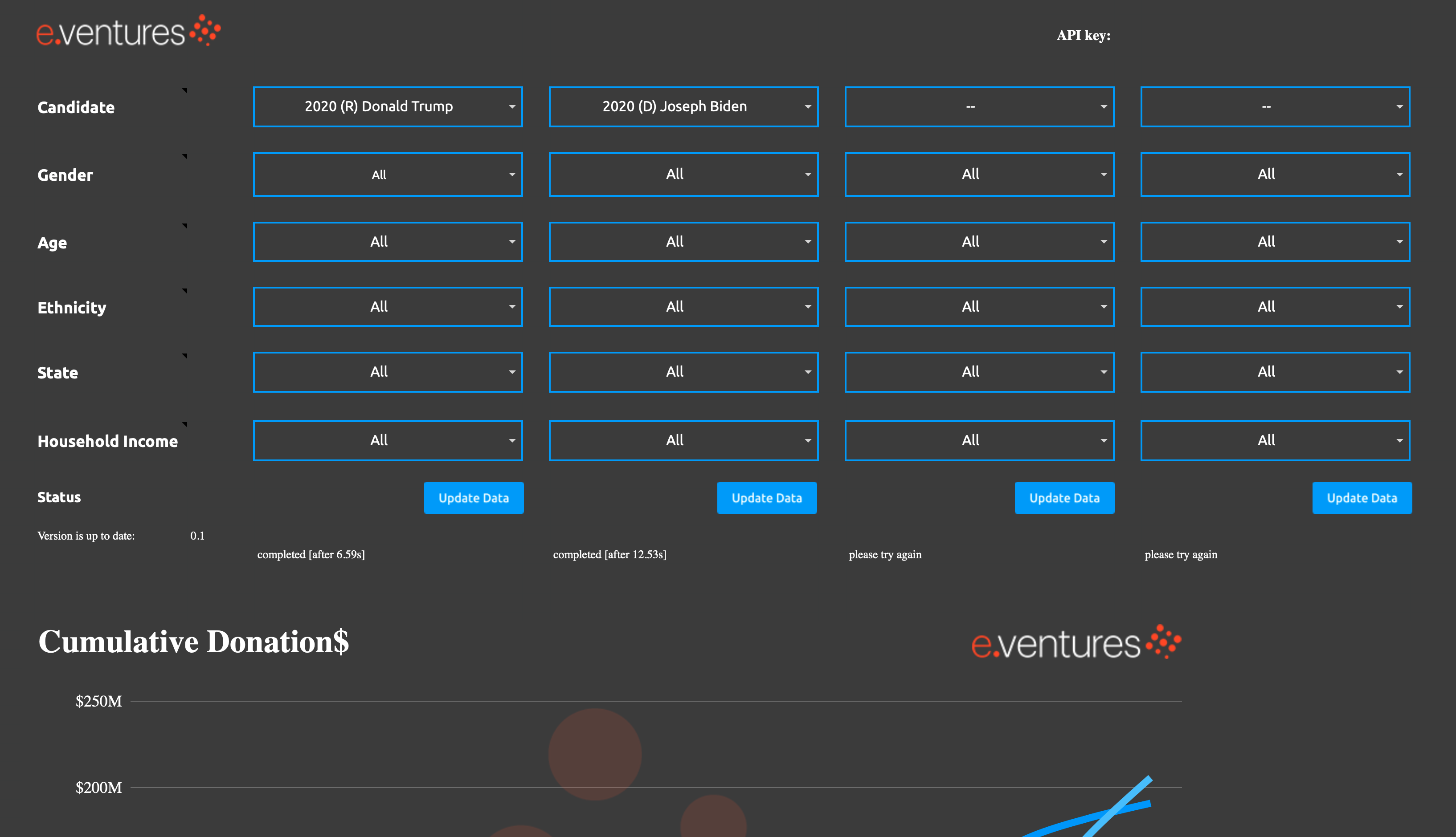
The Cohort Analysis Google Sheet compares contributions by candidates and, in this screenshot, selected age groups.
Donors and donations up to four candidates can be compared side by side. You can easily visualize the donation behaviour of different groups of gender, age, ethnicity, etc. Advanced derived features like the mean donor or donation amount retention can also give a deeper understanding of the donor's behaviour.
By clicking on the Update Data button, a SQL statement with the selected filters in the drop-down menus is run on the Elections SQL Interface, and up-to-date contribution data is imported into the Google Sheet. The sheet contains formulas to calculate features from the data and to display the results. Using the Google Sheet requires an API key that is inserted on the top of the chart sheet.
Note: The Cohort Analysis Google Sheet uses disclosed individual contribution data filed by the political committees and published by the FEC. Not all individual donor information are disclosed as there are thresholds for the requirements of disclosing donor information. The contributions by non-individuals (other political action groups (PACs) or organizations) are not included in the individual contribution data.
Therefore, the percentage of disclosed contributions versus the percentage of all contributions to a candidate can vary from around 60% to 95%. A direct comparison of contribution amounts between candidates does not reflect a comparison of the total contributions for the candidates.
Given this, relative comparisons of donors and donations are still possible, for example, between age groups of a candidate or over time.
Mapping the Contribution Data in the ObservableHQ Notebooks
The Elections data is enriched by location data (county name and FIPS code), as well as census tract and block codes. This allows the creation of map charts of the enriched individual contribution data.
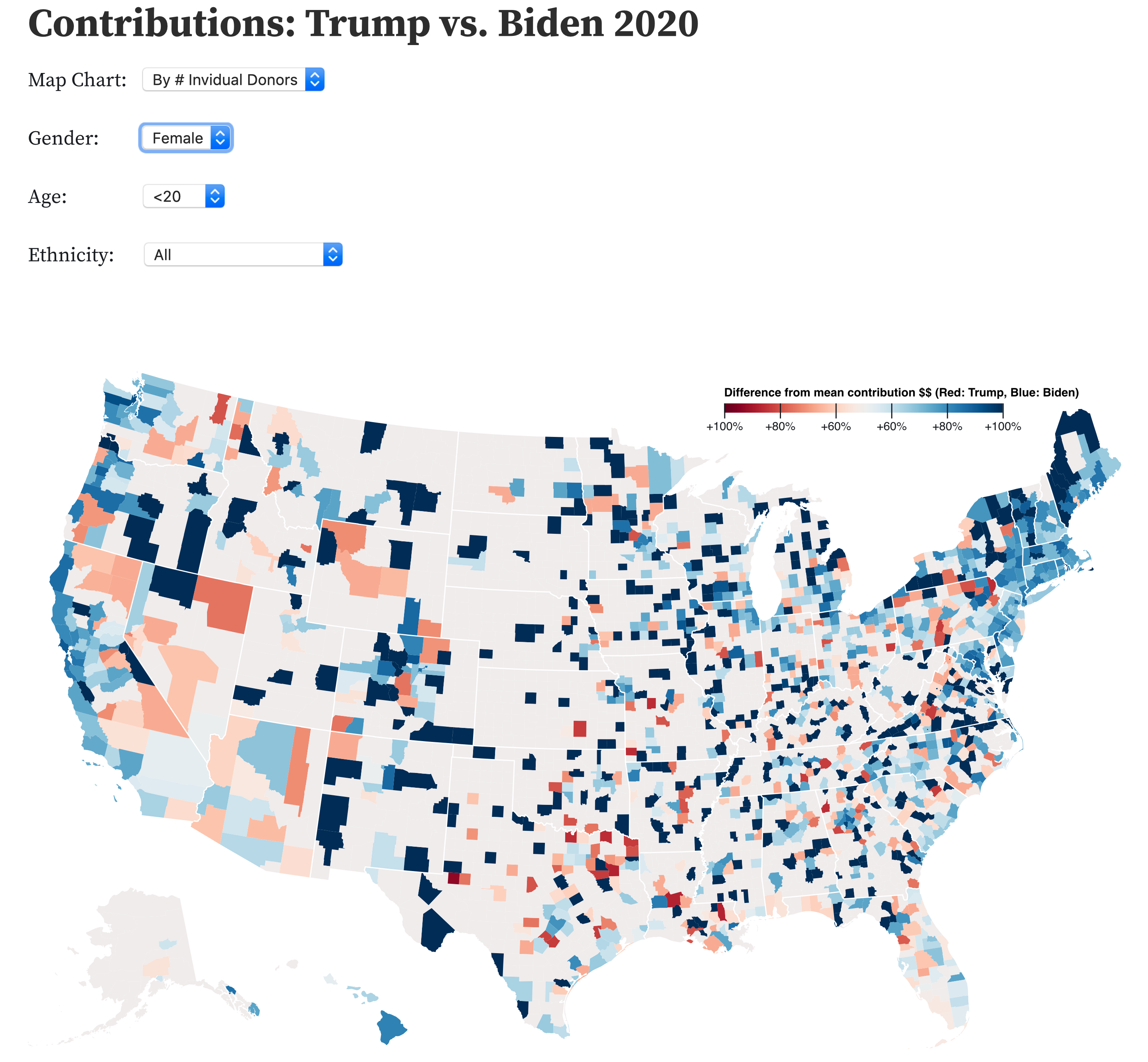
Here is an ObservableHQ notebook to map the sum of the collected contributions and the number of individual contributors for Trump and Biden in total or by a donor group sliced by gender, age and/or ethnicity.
Note that a direct comparison between candidates is not exact due to different percentages of disclosed individual donors.

ObservableHQ notebook with drop-down menus to slice and compare by donors' gender, age and ethnicity.
All the selections in the Google Sheet are translated into SQL queries inside the ObservableHQ notebook. The final SQL queries are then sent to the /query endpoint of the SQL Interface and the result is returned as a CSV file. The ObservableHQ notebook reads and processes the file and visualizes the result.
Note: Not all the data (e.g., individual contributions) can be enriched, due to missing or misspelled information (e.g., an incorrect street name). Also, not all data allows geocoding and can be included in the map chart.
Using the SQL Interface to Get the Data for Comparing Donors and Donations
The data used in the e.ventures Cohort Analysis Google Sheet and in the ObservableHQ is queried from the /query endpoint of the SQL Interface.
For example, here is the the SQL statement for loading the data for the ObservableHQ notebook above with the selected individual donor group of female donors under 20:
SELECT -- subquery 4
    CI.FIPS,
    COUNT(DISTINCT NAME_ID, ZIP_CODE)/TOTAL_BOTH AS PERCENTAGE
FROM ContributionsByIndividuals CI
     JOIN CommitteeMaster CM
         ON CI.CYCLE = CM.CYCLE AND
            CI.CMTE_ID = CM.CMTE_ID
     JOIN ( -- subquery 3
         SELECT FIPS, SUM(INDIVS) AS TOTAL_BOTH
         FROM (
             SELECT -- subquery 2
                 CMTE_ID,
                 FIPS,
                 COUNT( DISTINCT NAME_ID, ZIP_CODE) AS INDIVS
             FROM ContributionsByIndividuals
             WHERE CYCLE = 2020 AND
                   CMTE_ID IN (
                       SELECT CMTE_ID -- subquery 1
                       FROM CommitteeMaster
                       WHERE CYCLE = 2020 AND
                             CAND_ID IN ('P80001571', 'P80000722') -- subquery 1
                   ) AND
                   GENDER = 'F' AND
                   AGE < 20 AND
                   FIPS IS NOT NULL
             GROUP BY CMTE_ID, FIPS
         ) T -- subquery 2
         GROUP BY FIPS
     ) U -- subquery 3
     ON CI.FIPS = U.FIPS
WHERE CI.CYCLE = 2020 AND
      CAND_ID = 'P80000722' AND
      GENDER = 'F' AND
      AGE < 20
GROUP BY CI.FIPS; -- subquery 4
This SQL query appears to be quite complex at the first glance, as it consists of several nested subqueries. Each of those subqueries is easy to understand separately, so we will break those down in our explanation below.
The innermost subquery 1 fetches the committee ids for the candidates with the specified candidate Ids and is very similar to one of the examples above. Here, another subquery could be added to fetch the candidate for a name. Also, the election cycle of interest is given a part of the WHERE constraint.
Subquery 2 selects the sum of unique individual donors for each committee Id and FIPS county code. COUNT(DISTINCT NAME_ID, ZIP_CODE) defines an individual donor as the combination of the unique name (last name and first name) and zip code. This gives us the total number of unique donors for each county. Both the cycle and the committee Ids have to be specified. The donors that are taken into consideration are further filtered by setting gender and age constraints. Finally, the constraint FIPS IS NOT NULL ensures that contributions without a FIPS code are left out since they cannot be charted on the map. The GROUP BY clause defines the attributes for the COUNT aggregation.
Subquery 3 sums the unique donors for each committee up so that the individual donors are counted per committee. If one donor donates to Trump's committee and to Biden's committee, this will double count the donor, so that Biden and Trump both receive an equal score of 1/(1+1) = 50%, and sets the slider in the map chart above in the middle. Please also note that the above SQL query would have to be constructed differently if Trump and Biden had more principal campaign committees or authorized committees that they reported contributions for.
The outer query 4 finally calculates the share of Biden's individual donors by dividing his share by the total amount of individual donors from the red subquery. Trump's share of the total is 1 - (Biden's share). This query uses the JOIN statement to connect several required tables, one of them is the subquery 3 that produces a table-like result and can be joined as well. When performing a join, the attributes connecting equal datasets have to be specified in the ON statement. Also, the constraints on the donor group have to be repeated since we select each candidate's individual donors to calculate the share.
The final query gives a list of FIPS codes and percentages. 0% means that all of the individual donors (with an identifiable FIPS code) donate to Trump; 100% means that all of them contribute to Biden.
The user guide ends with this more complex SQL query that enables the user to design Charts and SQL queries on their own. This empowers you to gain deeper insights into the dynamics of individual donations and donor behavior.
Updated 8 days ago
